Estimate exposure time
Contents
Estimate exposure time#
import os
if not os.path.isfile("ECL-RSP-ARF_20211023T01.fits"):
    os.system("wget https://github.com/fcangemi/gp-tools-svom/raw/main/ECL-RSP-ARF_20211023T01.fits")
if not os.path.isfile("MXT_FM_PANTER_FULL-ALL-1.0.arf"):
    os.system("wget https://github.com/fcangemi/gp-tools-svom/raw/main/MXT_FM_PANTER_FULL-ALL-1.0.arf")
!pip install astropy
!pip install lmfit
Requirement already satisfied: astropy in /Users/fcangemi/opt/anaconda3/lib/python3.9/site-packages (5.1)
Requirement already satisfied: numpy>=1.18 in /Users/fcangemi/opt/anaconda3/lib/python3.9/site-packages (from astropy) (1.21.5)
Requirement already satisfied: pyerfa>=2.0 in /Users/fcangemi/opt/anaconda3/lib/python3.9/site-packages (from astropy) (2.0.0)
Requirement already satisfied: packaging>=19.0 in /Users/fcangemi/opt/anaconda3/lib/python3.9/site-packages (from astropy) (21.3)
Requirement already satisfied: PyYAML>=3.13 in /Users/fcangemi/opt/anaconda3/lib/python3.9/site-packages (from astropy) (6.0)
Requirement already satisfied: pyparsing!=3.0.5,>=2.0.2 in /Users/fcangemi/opt/anaconda3/lib/python3.9/site-packages (from packaging>=19.0->astropy) (3.0.9)
Requirement already satisfied: lmfit in /Users/fcangemi/opt/anaconda3/lib/python3.9/site-packages (1.1.0)
Requirement already satisfied: numpy>=1.19 in /Users/fcangemi/opt/anaconda3/lib/python3.9/site-packages (from lmfit) (1.21.5)
Requirement already satisfied: asteval>=0.9.28 in /Users/fcangemi/opt/anaconda3/lib/python3.9/site-packages (from lmfit) (0.9.28)
Requirement already satisfied: scipy>=1.6 in /Users/fcangemi/opt/anaconda3/lib/python3.9/site-packages (from lmfit) (1.9.1)
Requirement already satisfied: uncertainties>=3.1.4 in /Users/fcangemi/opt/anaconda3/lib/python3.9/site-packages (from lmfit) (3.1.7)
Requirement already satisfied: future in /Users/fcangemi/opt/anaconda3/lib/python3.9/site-packages (from uncertainties>=3.1.4->lmfit) (0.18.2)
from astropy.io import fits
import matplotlib.pyplot as plt
import numpy as np
from lmfit.models import ExpressionModel
from lmfit import minimize, Minimizer, Parameters, Parameter, report_fit
def read_arf(arf_filename):
    hdu1 = fits.open(arf_filename)
    arf_data=hdu1[1].data

    emin = arf_data.ENERG_LO
    emax = arf_data.ENERG_HI
    arf = arf_data.SPECRESP

    dE = emax - emin
    E = emin + (emax - emin) / 2

    return E, emin, emax, dE, arf

def bbody(x, phi0, kT):
    return phi0 * 8.0525 * x**2 / (kT**4 * (np.exp(x/kT) - 1))

def powerlaw(x, norm, Gamma):
    return norm * x**(-Gamma)

def cutoffpl(x, norm, Gamma, E_cut):
    return norm * x**(-Gamma) * np.exp(-x / E_cut)

#def powerlaw(params, x, data, error):
#    norm = params['norm']
#    Gamma = params['Gamma']
#    model = norm * x**(-Gamma)
#    return (model - data) / error

def function(x, a):
    return np.exp(- a * 1.5 / x ** 3)

def absorption():
    # From Strom & Strom 1961
    data = np.genfromtxt("absorption.txt", unpack = True, delimiter = ",",
                        skip_header = 1)
    wavelength = data[0]
    tau = data[1]
    norm_I = data[2]
    E = c.h * c.speed_of_light / (wavelength * 1e-10) * 6.242e15 # energy in keV
    plt.plot(E, norm_I, label = "data")
    plt.yscale("log")

    # Fit
    params, covs = curve_fit(function, E, norm_I, p0 = [0.50])
    print("params: ", params)

    plt.plot(E, function(E, params[0]), label = "Best fit")
    plt.ylim([1e-4, 1e1])
    plt.legend()
    plt.xlim([0, 2])

def plot_F(ax, E, F):
    ax.plot(E, F, color = "black", linewidth = 3)
    ax.set_xscale("log")
    ax.set_yscale("log")
    ax.set_xlabel("Energy [keV]")
    ax.set_ylabel("F(E) [ph/cm2/s/keV]")

def plot_EF(ax, E, EF):
    ax.plot(E, EF, color = "black", linewidth = 3)
    ax.set_xscale("log")
    ax.set_yscale("log")
    ax.set_xlabel("Energy [keV]")
    ax.set_ylabel("EF(E) [ph/cm2/s]")

def calculate_norm_from_flux(flux, Gamma, Emin, Emax):
    return flux * (-Gamma + 2) / (Emax**(-Gamma + 2) - Emin**(-Gamma + 2)) * 6.242e8

def calculate_flux_from_norm(norm, Gamma, Emin, Emax):
    return norm / (-Gamma + 2) * (Emax**(-Gamma + 2) - Emin**(-Gamma + 2)) / 6.242e8

def calculate_countrate(n_H, Eband, instrument, model, plot = 1):
    if(instrument == "MXT"):
        E, emin, emax, dE, arf = read_arf("MXT_FM_PANTER_FULL-ALL-1.0.arf")
    else:
        E, emin, emax, dE, arf = read_arf("ECL-RSP-ARF_20211023T01.fits")

    if((Eband[0] <= E[0] - dE[0]) or (Eband[-1] >= E[-1] + dE[-1])):
        print("ERROR: energy band outside the arf energy range !")
    else:
        E_r = E[(E>=Eband[0]) & (E<=Eband[1])]
        dE_r = dE[(E>=Eband[0]) & (E<=Eband[1])]
        arf_r = arf[(E>=Eband[0]) & (E<=Eband[1])]
        emax_r = emax[(E>=Eband[0]) & (E<=Eband[1])]
        emin_r = emin[(E>=Eband[0]) & (E<=Eband[1])]

        a = 0.286733

        if(model == "powerlaw"):
            F = norm * E_r**(-Gamma) * np.exp(- n_H * a / E_r**3)
            #print("Absorbed flux = ", sum(norm * E_r**(-Gamma) * np.exp(- n_H * a / E_r**3) * dE_r) / 6.242e8, "erg/s/cm2")
            countrate = sum(arf_r * norm * E_r**(-Gamma) * np.exp(- n_H * a / E_r**3) * dE_r)

        elif(model == "cutoffpl"):
            F = norm * E_r**(-Gamma) * np.exp(-E_r / E_cut) * np.exp(- n_H * a / E_r**3)
            countrate = sum(arf_r * norm * E_r**(-Gamma) * np.exp(-E_r / E_cut) * np.exp(- n_H * a / E_r**3) * dE_r)

        elif(model == "bbody"):
            F = norm * 8.0525 * E_r**2 / (kT**4 * (np.exp(E_r/kT) - 1)) * np.exp(- n_H * a / E_r**3)
            countrate = sum(arf_r * norm * 8.0525 * E_r**2 / (kT**4 * (np.exp(E_r/kT) - 1)) * np.exp(- n_H * a / E_r**3) * dE_r)

        else: # Brokenpowerlaw
            F = np.ones(len(E_r))
            countrate = 0
            for i in range(len(E_r)):
                if(E_r[i] <= E_break):
                    F[i] = norm * E_r[i]**(-alpha) * np.exp(- n_H * a / E_r[i]**3)
                    countrate += arf_r[i] * norm * E_r[i]**(-alpha) * np.exp(- n_H * a / E_r[i]**3) * dE_r[i]

                else:
                    F[i] = norm * E_r[i]**(-beta) * E_break**(beta - alpha) * np.exp(- n_H * a / E_r[i]**3)
                    countrate += arf_r[i] * norm * E_r[i]**(-beta) * E_break**(beta - alpha) * dE_r[i] * np.exp(- n_H * a / E_r[i]**3)
        if (plot == 1):
            fig = plt.figure(figsize = (7, 5))
            plt.plot(E_r, F, label = "Source", color = "red", linewidth = 3)
            plt.xscale("log")
            plt.yscale("log")
            plt.xlabel("Energy [keV]")
            plt.ylabel("ph/cm2/s/keV")
            #plt.ylim([0.01, 2])
        flux_simu = countrate / sum(arf_r * dE_r)
        return countrate, flux_simu

def calculate_background(instrument, Eband, plot = 1):
    a = 0.286733
    if(instrument == "ECLAIRs"):
        E, emin, emax, dE, arf = read_arf("ECL-RSP-ARF_20211023T01.fits")
    else:
        E, emin, emax, dE, arf = read_arf("MXT_FM_PANTER_FULL-ALL-1.0.arf")

    if((Eband[0] <= E[0] - dE[0]) or (Eband[-1] >= E[-1] + dE[-1])):
        print("ERROR: energy band outside the arf energy range !")
    else:
        E_r = E[(E>=Eband[0]) & (E<=Eband[1])]
        dE_r = dE[(E>=Eband[0]) & (E<=Eband[1])]
        arf_r = arf[(E>=Eband[0]) & (E<=Eband[1])]
        emax_r = emax[(E>=Eband[0]) & (E<=Eband[1])]
        emin_r = emin[(E>=Eband[0]) & (E<=Eband[1])]

        if(instrument == "ECLAIRs"):
            # 2SJPL Model from Moretti+2009
            Gamma_1 = 1.4
            Gamma_2 = 2.88
            E_B = 29             # keV
            norm = 0.109         # ph/cm2/s/keV/sr
            F = norm / ((E_r / E_B)**(Gamma_1) + (E_r / E_B)**(Gamma_2))
            countrate = sum(arf_r / (0.24 * 1024) * 0.16 * 0.3436 * 80 * 80 * norm / ((E_r / E_B)**(Gamma_1) + (E_r / E_B)**(Gamma_2)) * dE_r)

        else:
            # Powerlaw Model from Moretti+2009
            norm = 3.67e-3 * 65318 * (13.5*0.0002777)**2 #norm in ph/cm2/s/keV/deg2 * nb pixel contributing to the PSF * (13.5 arcsec/pixel)**2
            Gamma = 1.47
            F = norm * E_r**(-Gamma)
            #countrate = sum(arf_r * norm * E_r**(-Gamma) * dE_r)
            F = norm * E_r**(-Gamma) * np.exp(- n_H * a / E_r**3)
            countrate = sum(arf_r * norm * E_r**(-Gamma) * np.exp(- n_H * a / E_r**3) * dE_r)

        if(plot == 1):
            plt.plot(E_r, F, color = "blue", label = "CXB")
            plt.legend()
            plt.show()
    return countrate

def calculate_exposure(SNR, instrument, Eband):
    print("Emin  = ", Eband[0], "keV")
    print("Emax  = ", Eband[1], "keV")
    print("norm  = ", f'{norm:.4f}', "ph/s/cm2/keV")

    if(model == "powerlaw"):
        print("Gamma = ", Gamma)
    elif(model == "bknpowerlaw"):
        print("alpha = ", alpha)
        print("beta  = ", beta)
        print("E_break = ", E_break, "keV")
    elif(model == "bbody"):
        print("kT    = ", kT, "keV")
    else:
        print("Gamma = ", Gamma)
        print("E_cut = ", E_cut)
    print("n_H   = ", n_H, "e21 cm-2")

    source, flux_simu = calculate_countrate(n_H, Eband, instrument, model)
    if(instrument == "MXT"):

        background = calculate_background("MXT", Eband)
        exposure = (SNR  / source * np.sqrt(source + background))**2
    else:
        background = calculate_background("ECLAIRs", Eband)
        exposure = (SNR  / source * np.sqrt(source / 0.4 + background))**2 # Skinner+2008

    print("Background =", f'{background:.4f}', "c/s in the energy band", Eband, "keV.")
    print("Source =", f'{source:.4f}', "c/s in the energy band", Eband, "keV.")
    print(instrument, ": need an exposure time of", f'{exposure:.2f}', "seconds for a SNR =", SNR, "over the energy band", Eband, "keV.")


def make_spectra(instrument, nbins, tps_expo, title = " ", path_to_fig = " ", ylim1 = " ", ylim2 = " ", color = "black"):
    if(instrument == "ECLAIRs"):
        E = np.logspace(0.4, 2.15, nbins + 1)
    else:
        E = np.logspace(-1, 1, nbins + 1)

    print("norm  = ", f'{norm:.4f}', "ph/s/cm2/keV")

    if(model == "powerlaw"):
        print("Gamma = ", Gamma)
    elif(model == "bknpowerlaw"):
        print("alpha = ", alpha)
        print("beta  = ", beta)
        print("E_break = ", E_break, "keV")
    elif(model == "bbody"):
        print("kT    = ", kT, "keV")
    else:
        print("Gamma = ", Gamma)
        print("E_cut = ", E_cut)
    print("n_H   = ", n_H, "e21 cm-2")

    Emin = E[0:-1]
    Emax = E[1:]
    Ebin = Emax - Emin
    SNR = []
    countrate = []
    energy = Emin + (Emax - Emin) / 2
    flux_simu = []
    background = []
    error = []

    for emin, emax in zip(Emin, Emax):

        src, f_simu = calculate_countrate(n_H, [emin, emax], instrument, model, plot = 0)
        bkg = calculate_background(instrument, [emin, emax], plot = 0)
        err = np.sqrt(src * tps_expo)
        if(instrument == "ECLAIRs"):
            snr = src / np.sqrt(src / 0.4 + bkg) * np.sqrt(tps_expo) # for ECLAIRs
        else:
            snr = src / np.sqrt(src + bkg) * np.sqrt(tps_expo) # for MXT
        SNR.append(snr)
        countrate.append(src)
        flux_simu.append(f_simu)
        background.append(bkg)
        error.append(err)

    # PLOTS
    fig, ax = plt.subplots(figsize = (11, 5), nrows = 1, ncols = 2)
    fig.suptitle(instrument + "," + title + ", $t_{expo} =$" + str(tps_expo) + " s, \n" + model)
    yerr = np.asarray(error) / tps_expo
    #ax[0].errorbar(energy, countrate, xerr = Ebin / 2, yerr = yerr, color = "black")
    #ax[0].set_xscale("log")
    #ax[0].set_yscale("log")
    #ax[0].set_xlabel("Energy [keV]")
    #ax[0].set_ylabel("counts/s/keV")
    #if(ylim1 != " "):
    #    ax[0].set_ylim(ylim1)
    ax[0].plot(energy, SNR, 'o-', color = color)
    ax[0].set_xscale("log")
    #ax[0].set_yscale("log")
    ax[0].set_xlabel("Energy [keV]")
    ax[0].set_ylabel("SNR")

    a = 0.286733
    #flux_simu_err = yerr / countrate * flux_simu
    flux_simu_err = flux_simu / np.asarray(SNR)
    ax[1].errorbar(energy, flux_simu, # * np.exp(- n_H * a / energy**3),
                   xerr = Ebin / 2, yerr = flux_simu_err, fmt = ".",
                   label = "simulated spectrum", color = "black")

    idx = np.where(np.isnan(flux_simu_err) == False)[0]
    energy_g = energy[idx]
    flux_simu_g = np.asarray(flux_simu)[idx]
    flux_simu_err_g = flux_simu_err[idx]
    if(model == "powerlaw"):
        gmod = ExpressionModel("norm * x**(-Gamma) * exp(- n_H * 0.286733 / x**3)")
        params = gmod.make_params(norm = 1, Gamma = 2, n_H = 20.)
        params["n_H"].set(min = 0.1)
        params["n_H"].set(max = 120.)
        result = gmod.fit(flux_simu_g, params, x = energy_g, weights = 1. / flux_simu_err_g, scale_covar=False)
        ax[1].plot(energy, powerlaw(energy, result.params["norm"], result.params["Gamma"]) * np.exp(- result.params["n_H"] * 0.286733 / energy**3),
                  color = "red", linewidth = 3, label = "Best fit")

    elif(model == "cutoffpl"):
        gmod = ExpressionModel("norm * x**(-Gamma) * exp(-x / E_cut) * exp(- n_H * 0.286733 / x**3)")
        params = gmod.make_params(norm = 1., Gamma = 1.7, E_cut = 70., n_H = 20.)
        params["E_cut"].set(min = 1.)
        params["E_cut"].set(max = 500.)
        params["n_H"].set(min = 0.1)
        params["n_H"].set(max = 120.)
        result = gmod.fit(flux_simu_g, params, x = energy_g, weights = 1. / flux_simu_err_g, scale_covar=False, max_nfev = 10000)
        ax[1].plot(energy, cutoffpl(energy, result.params["norm"], result.params["Gamma"], result.params["E_cut"]) * np.exp(- result.params["n_H"] * 0.286733 / energy**3),
                  color = "red", linewidth = 3, label = "Best fit")

    elif(model == "bbody"):
        gmod = ExpressionModel("norm * 8.0525 * x**2 / (kT**4 * (exp(x/kT) - 1)) * exp(- n_H * 0.286733 / x**3)")
        params = gmod.make_params(norm = 1., kT = 1, n_H = 20.)
        params["norm"].set(min = 0.001)
        params["norm"].set(max = 10)
        params["kT"].set(min = 0.01)
        params["kT"].set(max = 3.)
        params["n_H"].set(min = 0.1)
        params["n_H"].set(max = 120.)
        result = gmod.fit(flux_simu_g, params, x = energy_g, weights = 1. / flux_simu_err_g, scale_covar=False, max_nfev = 10000)
        ax[1].plot(energy, bbody(energy, result.params["norm"], result.params["kT"]) * np.exp(- result.params["n_H"] * 0.286733 / energy**3),
                  color = "red", linewidth = 3, label = "Best fit")
    print(result.fit_report())

    ax[1].set_xscale("log")
    ax[1].set_yscale("log")
    ax[1].set_ylabel("ph/s/cm2/keV")
    ax[1].set_xlabel("Energy [keV]")
    ax[1].legend()
    #plt.title(instrument + "," + title + ", $t_{expo} =$" + str(tps_expo) + " s")
    if(ylim2 != " "):
        ax[1].set_ylim(ylim2)

    if(model == "powerlaw"):
        ax[1].set_title("norm   = " + str(result.params["norm"].value)[0:5] + " +/- " +
                        str(result.params["norm"].stderr)[0:5] + "\n"
                        "Gamma = " + str(result.params["Gamma"].value)[0:5] + " +/- " +
                        str(result.params["Gamma"].stderr)[0:5] +  "\n"
                        "n_H    = " + str(result.params["n_H"].value)[0:5] + " +/- " +
                        str(result.params["n_H"].stderr)[0:5] + "$\\times 10^{21}$ cm-2",
                        fontsize = 8)

    elif(model == "cutoffpl"):
        ax[1].set_title("norm   = " + str(result.params["norm"].value)[0:5] + " +/- " +
                        str(result.params["norm"].stderr)[0:5] + "\n"
                        "Gamma = " + str(result.params["Gamma"].value)[0:5] + " +/- " +
                        str(result.params["Gamma"].stderr)[0:5] +  "\n"
                        "E_cut = " + str(result.params["E_cut"].value)[0:5] + " +/- " +
                        str(result.params["E_cut"].stderr)[0:5] +  " keV \n"
                        "n_H    = " + str(result.params["n_H"].value)[0:5] + " +/- " +
                        str(result.params["n_H"].stderr)[0:5] + "$\\times 10^{21}$ cm-2",
                        fontsize = 8)

    elif(model == "bbody"):
        ax[1].set_title("norm   = " + str(result.params["norm"].value)[0:5] + " +/- " +
                        str(result.params["norm"].stderr)[0:5] + "\n"
                        "kT = " + str(result.params["kT"].value)[0:5] + " +/- " +
                        str(result.params["kT"].stderr)[0:5] +  " keV\n"
                        "n_H    = " + str(result.params["n_H"].value)[0:5] + " +/- " +
                        str(result.params["n_H"].stderr)[0:5] + "$\\times 10^{21}$ cm-2",
                        fontsize = 8)


    if(path_to_fig != " "):
        fig.savefig(path_to_fig + title + "_" + instrument + "_" + str(tps_expo) + "s_" + str(nbins) + "bins.pdf", bbox_inches = "tight")
This notebook uses ancillary response files of MXT and ECLAIRs in order to calculate the exposure time needed to achieve a signal to noise ratio given the spectrum of a source.
1. Choose the model and define parameters#
Four types of models can be used:
Simple powerlaw, “powerlaw”:#
\(\phi_0\): flux normalization at 1 keV in ph/cm2/s/keV, named “norm” in this notebook;
\(\Gamma\): photon index, named “Gamma” in this notebook.
NB: for this model, you can alternatively calculate the flux normalization \(\phi_0\) by calling calculate_norm_from_flux(unabsorbed_flux, Gamma, Emin, Emax) and giving the unabsorbed flux in ergs/cm2/s between Emin keV and Emax keV.
Broken powerlaw, “bknpowerlaw”:#
\(\phi_0\): flux normalization at 1 keV in ph/cm2/s/keV, named “norm” in this notebook;
\(E_\mathrm{break}\): break energy in keV, named “E_break” in this notebook;
\(\alpha\): photon index of the low energy powerlaw, named “alpha” in this notebook;
\(\beta\): photon index of the high energy powerlaw, named “beta” in this notebook.
Cutoff powerlaw, “cutoffpl”:#
\(\phi_0\): flux normalization at 1 keV in ph/cm2/s/keV, named “norm” in this notebook;
\(\Gamma\): photon index, named “Gamma” in this notebook;
\(E_\mathrm{cut}\): cutoff energy in keV, “E_cut” in this notebook.
Black body, “bbody”:#
\(\phi_0\): flux normalization: \(\phi_0 = L_{39}/D_{10}^2\), where \(L_{39}\) is the source luminosity in unit of \(10^{39}\) erg/s and \(D_{10}\) is the distance to the source in units of 10 kpc. (See https://heasarc.gsfc.nasa.gov/xanadu/xspec/manual/node137.html);
\(kT\): temperature in keV, name “kT” in this notebook;
For all the models, absorption is taken into account thanks to the hydrogen density column parameter n_H, in \(10^{21}\)cm\(^{-2}\).
2. Calculate the exposure#
Once you have defined your model and the corresponding parameters, you can call “calculate_exposure(SNR, instrument, Eband)” to calculate the exposure time needed. This function has three arguments:
“SNR”: Signal to Noise Ratio;
“instrument”: you can choose between “MXT” or “ECLAIRs”;
“Eband”: energy band for which you want to calculate the exposure time, [Emin, Emax], Emin and Emax in keV.
To edit the cells, click on the rocket at the top of this page, and then click on the "Live Code" button. Once your cell is edited you can click on "run" (the first time you are running, you may need to click on "restart & run all").
Few examples#
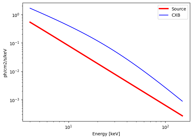
Powerlaw (example for the Crab)#
# Model and parameters
model = "powerlaw"
norm  = 10         # Flux normalisation in ph/cm2/s/keV
Gamma = 2.1        # Photon index
n_H   = 4.5        # Density column in 1e21 cm-2

# Exposure time
calculate_exposure(SNR = 10, instrument = "ECLAIRs", Eband = [4, 150])
Emin  =  4 keV
Emax  =  150 keV
norm  =  10.0000 ph/s/cm2/keV
Gamma =  2.1
n_H   =  4.5 e21 cm-2
Background = 3587.2578 c/s in the energy band [4, 150] keV.
Source = 523.9236 c/s in the energy band [4, 150] keV.
ECLAIRs : need an exposure time of 1.78 seconds for a SNR = 10 over the energy band [4, 150] keV.
Alternatively, you can give the unabsorbed flux to calculate the flux normalization:
unabsorbed_flux = 2.24e-8   # Unabsorbed flux in ergs/cm2/s between 2-10 keV
norm = calculate_norm_from_flux(unabsorbed_flux, Gamma, 2, 10)
calculate_exposure(SNR = 5, instrument = "MXT", Eband = [0.2, 10])
Emin  =  0.2 keV
Emax  =  10 keV
norm  =  10.0805 ph/s/cm2/keV
Gamma =  2.1
n_H   =  4.5 e21 cm-2
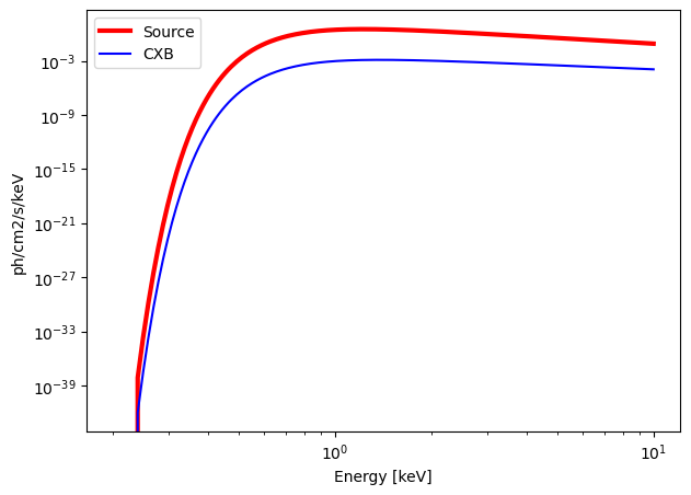
Background = 0.0594 c/s in the energy band [0.2, 10] keV.
Source = 131.8547 c/s in the energy band [0.2, 10] keV.
MXT : need an exposure time of 0.19 seconds for a SNR = 5 over the energy band [0.2, 10] keV.
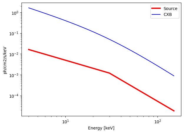
Broken Powerlaw#
model   = "bknpowerlaw"
norm    = 0.1           # Flux normalisation in ph/cm2/s/keV
E_break = 30            # Break energy in keV
alpha   = 1.3           # Photon index of the low energy powerlaw
beta    = 2.6           # Photon index of the high energy powerlaw
n_H     = 2.0           # Density column in 1e21 cm-2
calculate_exposure(SNR = 30, instrument = "ECLAIRs", Eband = [4, 150])
Emin  =  4 keV
Emax  =  150 keV
norm  =  0.1000 ph/s/cm2/keV
alpha =  1.3
beta  =  2.6
E_break =  30 keV
n_H   =  2.0 e21 cm-2
Background = 3587.2578 c/s in the energy band [4, 150] keV.
Source = 35.7848 c/s in the energy band [4, 150] keV.
ECLAIRs : need an exposure time of 2584.09 seconds for a SNR = 30 over the energy band [4, 150] keV.
Cutoff Powerlaw#
model = "cutoffpl"
norm  = 0.1         # Flux normalisation in ph/cm2/s/keV
E_cut = 40          # Energy cutoff in keV
Gamma = 1.7         # Photon index
n_H   = 0           # Density column in 1e21 cm-2
calculate_exposure(SNR = 10, instrument = "ECLAIRs", Eband = [4, 100])
Emin  =  4 keV
Emax  =  100 keV
norm  =  0.1000 ph/s/cm2/keV
Gamma =  1.7
E_cut =  40
n_H   =  0 e21 cm-2
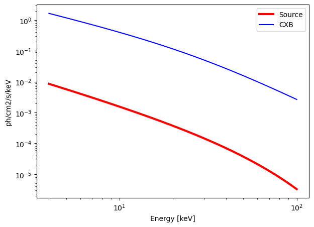
Background = 3569.5199 c/s in the energy band [4, 100] keV.
Source = 9.4439 c/s in the energy band [4, 100] keV.
ECLAIRs : need an exposure time of 4028.72 seconds for a SNR = 10 over the energy band [4, 100] keV.
Black Body#
model = "bbody"
norm  = 1.       # normalization
kT    = 0.5      # Black body temperature in keV
n_H   = 0.       # Density column in 1e21 cm-2

calculate_exposure(SNR = 7, instrument = "MXT", Eband = [0.2, 10])
Emin  =  0.2 keV
Emax  =  10 keV
norm  =  1.0000 ph/s/cm2/keV
kT    =  0.5 keV
n_H   =  0.0 e21 cm-2
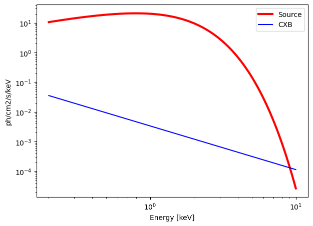
Background = 0.2285 c/s in the energy band [0.2, 10] keV.
Source = 957.6226 c/s in the energy band [0.2, 10] keV.
MXT : need an exposure time of 0.05 seconds for a SNR = 7 over the energy band [0.2, 10] keV.
Simulate your spectra#
First define your model parameters (works for powerlaw, cutoffpl, bbody):
model = "cutoffpl"
norm  = 10           # Flux normalisation in ph/cm2/s/keV
E_cut = 40          # Energy cutoff in keV
Gamma = 2.1         # Photon index
n_H   = 2           # Density column in 1e21 cm-2
Then define the parameters to compute the spectrum :
instrument: the instrument “MXT” or “ELCAIRs”
nbins: the number of energy bins you want for computing your spectrum
tps_expo: the exposure time (in seconds)
You can also define optionnal parameters:
title: a title for your figure (in string)
path_to_fig: the path where you want to save your figure (in string)
ylim1: limits for your y axis for the SNR VS Energy plot (for instance [1, 100])
ylim2: limits for your y axis for the spectrum (for instance [1e-6, 1])
color: the color you want to plot the SNR
Then you can run the simulation by calling the “make_spectra()” function.
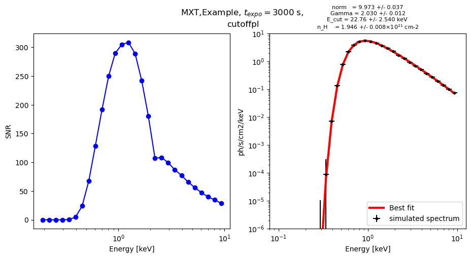
instrument = "MXT"
nbins = 32
tps_expo = 3000

# Optionnal parameters
title = "Example"
path_to_fig = " "
ylim1 = " "
ylim2 = [1e-6, 10]
color = "blue"

# Run make_spectra
make_spectra(instrument, nbins, tps_expo, title, path_to_fig, ylim1, ylim2, color)
norm  =  10.0000 ph/s/cm2/keV
Gamma =  2.1
E_cut =  40
n_H   =  2 e21 cm-2
[[Model]]
    Model(_eval)
[[Fit Statistics]]
    # fitting method   = leastsq
    # function evals   = 70
    # data points      = 28
    # variables        = 4
    chi-square         = 32.8502047
    reduced chi-square = 1.36875853
    Akaike info crit   = 12.4730970
    Bayesian info crit = 17.8019151
    R-squared          = 0.65331278
[[Variables]]
    norm:   9.97363429 +/- 0.03783086 (0.38%) (init = 1)
    Gamma:  2.03044528 +/- 0.01281399 (0.63%) (init = 1.7)
    E_cut:  22.7653706 +/- 2.54070426 (11.16%) (init = 70)
    n_H:    1.94643304 +/- 0.00811948 (0.42%) (init = 20)
[[Correlations]] (unreported correlations are < 0.100)
    C(Gamma, E_cut) = 0.944
    C(Gamma, n_H)   = 0.829
    C(norm, E_cut)  = -0.699
    C(E_cut, n_H)   = 0.692
    C(norm, Gamma)  = -0.475
/var/folders/cf/lj06vg8d24d6_0gnzr5lh2d40000gn/T/ipykernel_18190/136565042.py:235: RuntimeWarning: invalid value encountered in double_scalars
  snr = src / np.sqrt(src + bkg) * np.sqrt(tps_expo) # for MXT